gbspy.fits module

Provide commonly used fitting profiles.

class gbspy.fits.FitConfig(fun, **kwargs)

Bases: object

Fit configuration object

Holds arguments to call scipy.optimize.curve_fit() with.

fun

Target profile to fit as a callable object.

Type: callable

opts

Dictionnary containing keyword-arguments that will be passed to the scipy routine.

Type: dict

update_fit_opts(**new_opts)

Update kwargs options

This will call the underlying dict.update() on the options stored by the class. Existing options will be replaced, additional arguments will create new options.

Parameters: **new_opts (dict, optional) – Options to add or update, which must be accepted by curve_fit().
Returns: The updated FitConfig object.
Return type: FitConfig

gbspy.fits.ffun_double_exp(x, q0, x0, L_left, L_right)

Double exponential profile

This profile is characterized as

\[ \begin{align}\begin{aligned}f(x) = q_0 \exp(-(x-x_0)/L(x)),\\\begin{split}L(x) = \begin{cases} L_{\text{left}}, & \text{if}\ x<x_0 \\ L_{\text{right}}, & \text{otherwise} \end{cases}\end{split}\end{aligned}\end{align} \]

Parameters

x (array_like) – Input data.
q0 (float) – Multiplicative constant.
x0 (float) – Point at which the decay length of the profile changes.
L_left (float) – Decay lengths of the profile.
L_right (float) – Decay lengths of the profile.

Returns

The profile evaluated at x.

Return type

array_like

gbspy.fits.ffun_eich2011(x, q0, L, S, qb)

Convolution of an exponential profile and a Gaussian function

This profile is proposed by Eich et al. as the result of a competition between parallel plasma transport along a divertor leg and perpendicular diffusion (leakage) into the private flux region, assuming an exponential profile at the divertor entrance. A convolution between an exponential profile and exponential is proposed to model this process:

\[f(x) = \frac{q_0}{2} \exp\left(\frac{S^2}{4L^2} - \frac{x}{L}\right) \mathrm{erfc}\left(\frac{S}{2L} - \frac{x}{S}\right) + q_{\text{BG}}\]

where \(S\) the width of the Gaussian and \(L\) the decay length of the exponential profile. See equation (2) in Eich et al. (2011).

Parameters

x (array_like) – Input data.
q0 (float) – Multiplicative constant and background flux
qb (float) – Multiplicative constant and background flux
L (float) – Width of the exponential and Gaussian profiles.
S (float) – Width of the exponential and Gaussian profiles.

Returns

The profile evaluated at x.

Return type

array_like

gbspy.fits.ffun_exp(x, q0, L)

Exponential profile

Defined by

\[f(x) = q_0 \exp(-x/L)\]

Parameters

x (array_like) – Input data.
q0 (float) – Multiplicative factor and decay length of the exponential profile.
L (float) – Multiplicative factor and decay length of the exponential profile.

Returns

The exponential profile evaluated at x.

Return type

array_like

gbspy.fits.ffun_gaussian(x, q0, x0, L)

Gaussian function

Defined as:

\[f(x) = q_0 \exp\left(\frac{-(x-x_0)^2}{2L^2}\right)\]

Parameters

x (array_like) – Input data.
q0 (float) – Multiplicative constant
x0 (float) – Center and width of the peak.
L (float) – Center and width of the peak.

Returns

The Gaussian evaluated at x.

Return type

array_like

gbspy.fits.ffun_linear(x, a, b)

Linear profile

Returns the result of evaluating

\[f(x) = ax + b\]

Parameters

x (array_like) – Input data.
a (float) – Slope and height of the profile
b (float) – Slope and height of the profile

Returns

The linear profile evaluated at x.

Return type

array_like

gbspy.fits.fit(f, xdata, ydata, return_func=None, **kwargs_scipy)

Non-linear least square fitting wrapper

This function wraps calls to scipy.optimize.curve_fit(). In addition to scipy’s routine, this function accepts a string as first argument to reference commonly used fitting profiles.

When the first argument is a callable, this routine behaves like like scipy’s curve_fit().

When the first argument is a string:

optional arguments accepted by scipy’s routine (such as bounds or p0) may be set automatically. You can override their values by passing them directly to fit() yourself. You can see which parameters are set by calling get_fit_configuration(),
unless specified otherwise, the fitting function is also returned (as the last return value).

Parameters

f (callable or str) –
If string, the following options are accepted:
- "linear": Linear function,
- "exp": Exponential decay,
- "doubleexp": Double exponential decay,
- "gaussian": Gaussian function,
- "eich2011": see ffun_eich2011().
return_func (bool, optional) – Whether to return the fitting function. True if f is a string, False otherwise.
kwargs_scipy (dict, optional) – Any keyword argument accepted by curve_fit().

Returns

popt (array) – See curve_fit().
pcov (2-D array) – See curve_fit().
func (callable) – The function that was used to fit the curve. This argument is only returned when the first argument is a string, or when explicitely enabled by the caller.

Examples

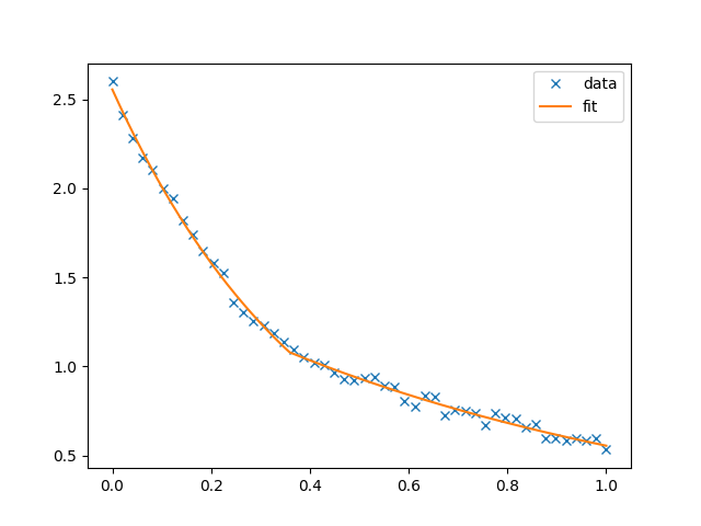
Generate a noisy double exponential profile: two decay lengths of 0.4 and 0.95 are considered. The transition between the decay lengths occurs at x=0.3678:

In [1]: import gbspy.fits as fits

In [2]: x = np.linspace(0, 1, 50)

In [3]: y_true = fits.ffun_double_exp(x, 1.0, 0.3678, 0.4, 0.95)

In [4]: noise = 1e-1 * np.random.random((50, ))

In [5]: y = y_true + noise

Fit the curve. Here, we provide a reasonable guess of 0.5 at which the decay length changes,

In [6]: params, cov, ffun = fits.fit("doubleexp", x, y, p0=[1.0, 0.5, 1.0, 1.0])

In [7]: print(
   ...:     (
   ...:         f"First decay length: {params[2]!r}\n"
   ...:         f"Second decay length: {params[3]!r}\n"
   ...:         f"Transition at: {params[1]!r}"
   ...:     )
   ...: )
   ...: 
First decay length: 0.4161962043210802
Second decay length: 0.9621985264070205
Transition at: 0.35874387625916493

This yields a reasonable estimate of the parameters. We can also plot the result of the fit with

In [8]: import matplotlib.pyplot as plt

In [9]: plt.figure()
Out[9]: <Figure size 640x480 with 0 Axes>

In [10]: plt.plot(x, y, "x", label="data")
Out[10]: [<matplotlib.lines.Line2D at 0x7f0ac485a940>]

In [11]: xhres = np.linspace(0, 1, 2000)

In [12]: plt.plot(xhres, ffun(xhres, *params), label="fit")
Out[12]: [<matplotlib.lines.Line2D at 0x7f0ac485abb0>]

In [13]: plt.legend()
Out[13]: <matplotlib.legend.Legend at 0x7f0ac48c4cd0>

gbspy.fits.get_fit_configuration(name, x, y)

Returns fitting options based on input data

Given the name associated with a given profile, returns both a callable for this profile and fitting options. The fitting options must be accepted by scipy.optimize.curve_fit().

Parameters

name (str) – Name associated to the profile that must be fit (for example, "linear").
x (array_like or object) – Data points to be fitted, accepted by scipy’s curve_fit().
y (array_like or object) – Data points to be fitted, accepted by scipy’s curve_fit().

Returns

An object storing the callable associated to the requested profile and options to pass to curve_fit().

Return type

FitConfig